Systems simulation · ASELSAN internship · 2026
CPU Scheduler Simulator
Round Robin, MLFQ, CFS and aging priority on the same workload, measured by one accountant that has never heard of any of them.
Why I built it
This task wasn’t actually going to be mine. I kept begging my mentor for a C++ project, and in the end the team talked it over and told me to build a scheduler. I was really excited when I heard it: it was a chance to learn how the algorithms from our OS course are actually implemented, and how algorithms far more complex than the ones in that course work.
What it is
A CPU scheduling comparison harness I built during my internship on ASELSAN’s embedded systems team. It has one simulation engine, interchangeable scheduling policies, and a single set of metrics computed the same way for all of them, so the comparison is fair.
The founding rule is that no algorithm may see the future. A policy is told only what has already happened: who arrived, who has been waiting, how much CPU each job has used. That’s the standard a real scheduler is held to, and it’s why Shortest Job First isn’t here while MLFQ and CFS are.
The pieces
- Driver Owns the loop and decides how time moves.
- advance
- Kernel Wakes only when something can change: charges elapsed time, notices what finished, records every event.
- who runs next?
- Policy Has no clock and no power to act. It only answers.
- Event trace One CSV row per event, in order: seq, time, event, job, cpu.
- read afterwards
- Accountant Turns the trace into metrics. It has never heard of any algorithm.
- checked against
- Animation Manim draws the same trace and refuses to draw a chart that disagrees with the numbers.
Round Robin, MLFQ, CFS and aging priority each live in one file and register themselves by name, so a run picks its algorithm with a string. Because the accountant only reads the trace, adding a new algorithm never needs a new metric, and adding a metric never touches an algorithm.
Checking the numbers
Between arriving and finishing, a job is always in exactly one state: waiting, running, blocked
on I/O, or being switched in. So for every finished job, turnaround = waiting + CPU + I/O + switch overhead must hold exactly. It’s a
conservation law rather than an estimate, and the strongest check on the whole pipeline: if it
fails, blocked time is being counted as waiting time somewhere. All numbers are integer ticks
until the last division, so results are exact and reproducible. The project has 84 Catch2
tests.
One workload, five runs
| Run | Avg response | Avg waiting | Avg turnaround | CPU use | Context switches |
|---|---|---|---|---|---|
| RR, quantum 2 | 3.17 | 22.50 | 35.00 | 98% | 28 |
| RR, quantum 8 | 8.83 | 21.83 | 34.33 | 96% | 16 |
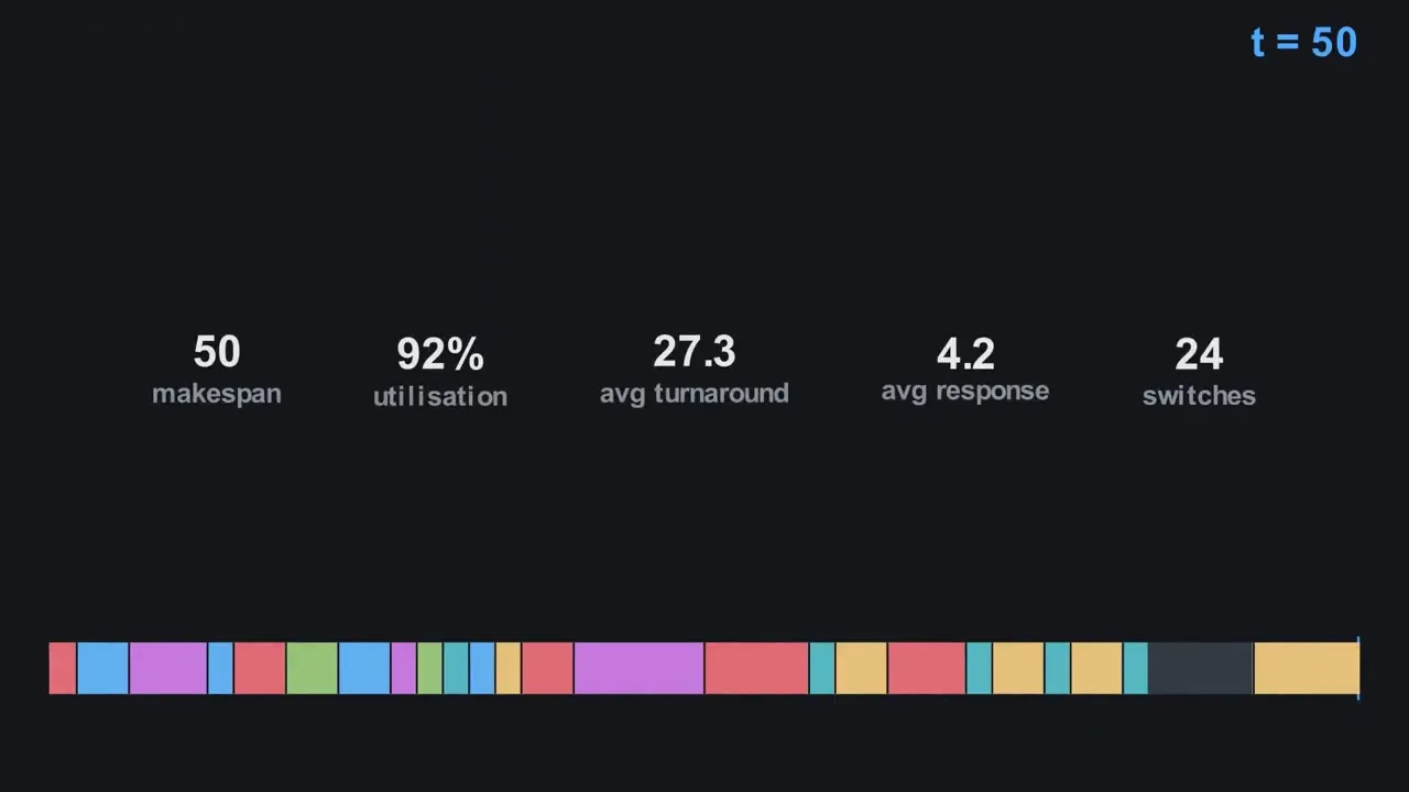
| Aging priority | 4.17 | 14.83 | 27.33 | 92% | 24 |
| MLFQ | 2.83 | 21.50 | 34.00 | 100% | 28 |
| CFS | 1.50 | 18.17 | 30.67 | 92% | 30 |
Averages in ticks over one six-job workload, mixing CPU-heavy and I/O-heavy jobs. RR is Round Robin. Best value per column in bold. With one workload this shows trade-offs, not a winner.
Even this small workload shows the trade-offs. CFS gets every new job onto the CPU fastest. Aging priority finishes jobs soonest on average. Raising Round Robin’s quantum from 2 to 8 cuts context switches from 28 to 16, but nearly triples the average response time.
The animation
The video above is rendered with Manim (Python) straight from the simulator’s output. Nothing is invented at render time: each scene reads the trace files, and the loader cross-checks every trace against its recorded metrics before drawing. It walks through the six jobs, why they can’t all be satisfied at once, each algorithm in turn, and a final scoreboard.